Money as a Medium of Exchange in an Economy with Artificially Intelligent Agents
Abstract
We study the exchange economies of Kiyotaki & Wright (1989) in which agents must use a commodity or fiat money as a medium of exchange if trade is to occur. Our agents are artificially intelligent and are modeled as using classifier systems to make decisions. In the assignment of credit within the classifier systems, we introduce some innovations designed to study sequential decision problems in a multi-agent environment. For most economies that we have simulated, trading and consumption patterns converge to a stationary Nash equilibrium even if agents start with random rules. In economies with multiple equilibria, the only equilibrium that emerges in our simulations is the one in which goods with low storage costs play the role of medium of exchange (i.e., the ‘fundamental equilibrium’ of Kiyotaki and Wright).
1. Introduction
Kiyotaki & Wright (1989) studied how three classes of rational agents would interact within a Nash-Markov equilibrium in a world of repeated ‘Wicksell triangles’. This paper studies how a collection of artificially intelligent agents would learn to coordinate their activities if they were thrust into the economic environment described by Kiyotaki and Wright. Our agents’ behavior is determined by Holland (1975) classifier systems.[1]
Thus, while Kiyotaki and Wright studied stationary equilibria in which beliefs about ‘media of exchange’ are consistent with trading patterns, we study economies in which particular commodities emerge as media of exchange. We also study an economy (Economy C) in which a good from which no agent derives utility emerges as fiat money. We want to learn whether our artificially intelligent agents can learn to play a Markovian Nash equilibrium of the Kiyotaki-Wright model. When there are multiple Nash equilibria (e.g., the ‘fundamental’ and ‘speculative’ equilibria of Kiyotaki and Wright), we want to know whether the system might converge to some but not others of these equilibria. In addition, if classifier systems do converge to Nash-Markov equilibria, they might be used to compute equilibria in other economies for which it is difficult to obtain analytic solutions. To this end, we also study enlarged versions of the Kiyotaki-Wright model.
A classifier system is a collection of potential decision rules, together with an accounting system for selecting which rules to use. The accounting system credits rules generating good outcomes and debits rules generating bad outcomes. The system is designed to select a ‘co-adaptive’ set of rules that work well over the range of situations that an agent typically encounters. In a multiple-agent environment like Kiyotaki and Wright’s, the range of situations encountered by one agent depends on the actions taken by other agents. This means that the collections of rules used by the collection of agents must co-adapt jointly.
We study two sorts of classifier systems, with the distinction between them being induced by the fact that for many problems enumerating all possible rules would require a very long list. The first kind of classifier system is one in which a complete enumeration of all possible rules is carried along. For many problems, it is not feasible to use a complete enumeration classifier system because the state and action spaces are so large that the set of all possible rules is much too big. For us, a complete enumeration is tractable because the Kiyotaki-Wright model has low-dimensional state and action spaces.
The second kind of classifier system is designed for situations in which it is not efficient to carry along a complete enumeration of decision rules. In this case, a modified version of the genetic algorithm of Holland is used as a device for periodically eliminating some rules and injecting new rules into the population of rules to be operated on by the accounting system. The genetic-algorithm version of the classifier models learning in the face of unforeseen contingencies. When an unprecedented state arises which is not covered by the existing set of rules, the system contains a procedure for manufacturing and experimenting with new rules that apply in the new situation. Even though it is feasible for us to work with a complete enumeration of rules, we also study the genetic-algorithm version of the classifier.[2]
In this paper, we set up classifier systems for the Kiyotaki-Wright environment and simulate them on a computer. We also formulate definitions of equilibrium and stability for classifier systems, and pose some convergence questions. Although we suggest possible convergence theorems, we prove no theorems in this paper. 2. The Kiyotaki-Wright Environment describes the Kiyotaki-Wright environment. 3. Classifier Systems for the Kiyotaki-Wright Environment describes the classifier systems without genetics. 4. Classifier Systems for Supporting Kiyotaki and Wright’s Stationary Equilibria describes behavior in the stationary equilibria of Kiyotaki and Wright and also the types of classifier systems that could support that behavior. 5. Concepts of Convergence for Classifier Systems Playing Games defines stability criteria for sets of classifier systems, and discusses how these definitions can be used to formulate questions about whether systems of classifier systems converge to a stationary equilibrium. 6. Incomplete Enumeration Classifiers and the ‘Genetic Algorithm’ describes classifier systems operating with genetics. 7. Simulation Results describes our simulations of systems of classifier systems. In addition to the economies studied by Kiyotaki and Wright (including one with fiat money), we study an economy with five types of agents and five goods. 8. Conclusions concludes the paper.
2. The Kiyotaki-Wright Environment
There are three types of agents, with types being indexed by . Type agents get utility only from consuming type good. Type agent has access to a technology for producing type good, where . We initially specify according to Kiyotaki-Wright’s ‘model A’, namely, as follows:
| 1 | 2 |
| 2 | 3 |
| 3 | 1 |
This specification assumes no ‘double coincidence of wants’ and seems to call for a multilateral trading arrangement. All goods are indivisible. Each agent can store one and only one unit of only one good from one period to the next. When an agent of type consumes good at time , he immediately produces good , which he carries over to the next period. The net utility to an agent of type of consuming good and producing good is given by . We assume that an agent of type does not know his utility function, but does recognize utility when he experiences it. The goods are costly to store. Storing good () from to imposes costs at of . Following Kiyotaki and Wright, we assume that . We summarize this cost function by saying that is the one-period cost of storing one unit of good . We assume that individuals do not know this cost function, but that they do recognize costs when they bear them.
The economy and each agent within it live forever. There are large and equal numbers of agents of each type. We modify Kiyotaki and Wright’s model by assuming that each agent cares about his long-run average level of utility. (Kiyotaki and Wright assumed that agents have preferences ordered by expected discounted future utilities.) Each period, there is a random matching process that assigns each and every agent in the economy to a pair with one and only one other agent in the economy. The random matching technology matches agents without regard to type. Only pairs of agents matched together can trade at a point in time.
The economy begins at with agents being endowed with an arbitrary and randomly generated initial distribution of holdings of goods. At each date , each agent has to make two decisions sequentially. First, given the good he is holding and given the good held by the partner with whom he is matched at , he must decide whether to propose to trade. Trade occurs only if both parties propose to do so. Second, the agent must decide whether or not to consume the good with which he exits the trading process. If he doesn’t consume, he simply carries the good into period , experiencing cost . If an agent of type does consume good at , he experiences net utility , produces good , and experiences carrying costs . We assume that if and . We follow Kiyotaki and Wright both in adopting their specification of the physical environment and in considering only Markov strategies, but we drop the assumption of rational agents. Instead, our agents are assumed to be ‘artificially intelligent’, in the sense that they use versions of the classifier system introduced by Holland (1986).
Before describing the classifier systems used by our agents, we introduce some notation for naming agents and for describing the state of each individual agent in the economy. There is a collection of agents . A typical element of is denoted . Kiyotaki and Wright assumed that there was a continuum of each type of agent, while we assume that there is a finite number of each type. The first agents are of type I, the next are of type II, and the following are of type III. Here .
At the beginning of time , agent is carrying good . The variable characterizes the pre-match state of agent at time . There is a random matching process which each period matches each agent with a distinct agent . For each agent in each period, the matching process induces a function . After the matching process, the pre-trade state of agent is . The pair records what agent is carrying and what the agent with whom is matched at is carrying.
At , after being matched with agent , agent decides whether or not to propose to trade. We let denote the trading decision of agent at time , where
Similarly, summarizes the trading decision of the agent with whom is paired at . Trade takes place if and only if .
Let denote the post-trade (but pre-consuming decision) holdings of agent at . We then have that
After leaving the trading process with holdings , agent must decide whether to consume or to carry it into the next period. We let denote the consumption decision of agent at where
If agent decides to consume, he automatically produces good , which he carries into . From the specification of as a function of described above for Kiyotaki and Wright’s model A, we have that is a good of type 2 if is a type I agent, is a good of type 3 if is a type II agent, and is a good of type 1 if is a type III agent. It follows that beginning-of-period holdings of at time are described by[3]
3. Classifier Systems for the Kiyotaki-Wright Environment
We now describe the classifier systems that agents use to make their trading and consumption decisions.[4] Agents sequentially use two interconnected classifier systems each period. A first trading classifier system receives input in the form of the pre-trade state . This classifier system determines the trading decision , which interacts with the trading decision of the agent with whom is paired at to determine [see eq. (2)]. A second consumption classifier system takes as input and determines the consumption decision . The two classifier systems are used sequentially in this way each period, and their accounting systems are interconnected in ways to be described below.
A classifier system consists of the following objects:
A collection of trinary strings, called ‘classifiers’.
A system for interpreting or decoding the strings or classifiers as instructions mapping states into decisions. The first part of a string encodes a particular state or condition, while the second part encodes a particular action. Thus, an individual classifier or string is just an encoding of a single (state, action) pair. For a given state, there can be many classifiers present in a classifier system.
A list of ‘strengths’ attached to each classifier at each point in time
A system for reading in external messages or ‘states’ and for determining the set of classifiers that are pertinent, i.e., the set of classifiers whose ‘conditions’ are satisfied or ‘matched’ at that state. For a given state, the system can sometimes contain several classifiers with distinct actions.
An ‘auction system’ for determining which of the pertinent classifiers is allowed to make a decision at . Among all classifiers whose condition part matches the actual state at , the ‘highest bidder’ in the auction actually ‘makes the decision’ in real time.[5]
An accounting system for updating the strengths of the collection of classifiers in response to the net rewards that flow into the system as a result of the decisions that are made.
And possibly:
A genetic algorithm for introducing new strings and extinguishing old strings. This algorithm will be called whenever states are encountered for which no existing classifiers have their conditions met. The algorithm may also be applied from time to time as a device to promote experimentation.
We now describe each of these elements as applied to the Kiyotaki-Wright environment. We first consider an exchange classifier system, which maps the pre-trade state into a trading decision. This classifier system consists of a list of trinary strings of length 7. The first three digits represent own storage, the next three represent trading partner’s storage, and the seventh represents the trading decision.
Table 1:Encoding of goods in classifiers
Code | Meaning |
|---|---|
1 0 | Good 1 |
0 1 | Good 2 |
0 0 | Good 3 |
0 # | Not good 1 |
0¶ | Not good 2 |
¶ | Not good 3 |
The coding is written in the trinary alphabet , where means ‘don’t care’. For the trading decision, the code is in the binary alphabet , where 1 means trade, while 0 means don’t trade.
To illustrate how the codes in Table 1 are applied to encode particular trading classifiers, we consider the following two classifiers:
| Own storage | Partner storage | Trading decision |
|---|---|---|
| 1 0 0 | 0 0 1 | 1 |
| 1 0 0 | # # 0 | 0 |
The first classifier instructs an agent who is carrying good 1 and who is matched with someone carrying good 3 to offer to trade. The second classifier instructs an agent who is carrying good 1 not to trade if he is matched with someone who is not carrying good 3.
The exchange classifier system of agent consists of a list of such classifiers. Let index this collection of classifiers. A given classifier system has a fixed number of classifiers. For the exchange classifier system, how many distinct classifiers are possible? Evidently, . However, most of these classifiers are redundant in the sense that only a subset of them is needed to represent all possible trading decision rules defined on the state space when there are three goods. All rules can be written in terms of pairs of conditions drawn from Table 1. Thus, only strings are required to represent the complete set of possible rules for this system.
Assigned to each exchange classifier is a strength, denoted . The strength evolves over time in a way determined by the accounting system. The strengths attached to classifiers are used to determine the decisions made by the classifier system at . For a given state or ‘condition’ , there is a collection of classifiers within the classifier system whose conditions are satisfied. We denote the set of such classifiers by , defined as
The members of form a class of potential ‘bidders’ in an ‘auction’ whose purpose is to determine which classifier makes the decision of agent at time . When state is encountered at time by agent , the classifier belonging to that has the highest strength makes the decision. Let denote the index of the classifier to be used in deciding whether to trade at . Then,
We denote the action (trade or no trade) taken by classifier as . Equations (5) and (6) describe the ‘auction system’ by which the highest strength rule that applies in a given state is given the right to decide for agent at .
Because the trade and consumption classifier systems will be making payments to one another, we have to describe the consumption classifier system before describing the accounting system that updates strengths of the trade classifier system. The consumption classifier system is a collection of trinary strings of length 4. The first three positions encode using the same code that was described in Table 1. The condition part of the strings is written in terms of the trinary alphabet . The fourth position of a consumption string is the ‘action’ part, taking values of 1 (meaning consume) and 0 (meaning don’t consume).
We let consumption classifier strings be indexed by . The strength assigned to classifier of agent is . By virtue of eq. (2), the state can be expressed in terms of . Therefore it suffices to denote the set of ‘matched’ classifiers by , where
Let denote the classifier that makes the consumption decision at . The highest-strength classifier gets to make the decision:
Given the decisions determined by (6) and (8), evolves according to the law of motion (4).
3.1 Counters and Strength Evolution
We attach to each exchange classifier a ‘counter’ which records the cumulative number of times that classifier has won the auction as of date . We shall change the strength of classifier only when it actually wins the auction and thereby gets to make the exchange decision, which is why we need the counter . The counter for classifier is defined recursively in terms of the indicator , which records whether classifier wins the auction:
Notice that we initialize the counter of each classifier at unity. The strength of classifier at will be represented as .
Similarly, we attach to each consumption classifier a ‘counter’ which records the cumulative number of times that classifier has won the auction as of date . The counter is defined by
The strength of classifier at will be represented as .
3.2 Bid Functions and Strength Updates
The counters and induce a transformation of time in terms of which the strengths of classifiers and are updated. At date , a strength is attached to classifier , while a strength is attached to classifier of agent . At date , if classifier ’s condition is matched [i.e., if ], then classifier makes a bid of , where is a positive fraction that can depend on . If classifier wins the auction, its bid will be deducted from its strength. The winning bid will be allocated to augment the strength of other classifiers whose actions drove the system to the state that satisfied ’s condition. We choose the particular bid function
where and are positive constants adding up to less than one, and is a fraction which is proportional to the specificity of a particular classifier. In particular, we choose . Similarly, we define a function with . By the above choices of and , we favor specific rules over more general rules that can be activated by a particular state. When , classifier makes a bid of .
Only winning classifiers pay their bids by having them deducted from their strengths. The bid of the winning exchange classifier at is paid to the winning consumption classifier at , which is the classifier that is to be credited with setting the time state to . The bid of the winning consumption classifier at is paid to the winning exchange classifier at time , which is to be credited with setting the post-exchange state at at , thereby giving the winning consumption classifier a chance to bid.
We represent these payments in terms of the following difference equations:
In (14), is the external payoff when the winning consumption classifier makes final consumption decision . If the post-exchange state at is , then we have
There are several features of (14) and (15) that bear emphasizing. First, these are recursive formulas that make and averages of past payoffs (external rewards plus bids received from other classifiers) minus payments (bids made to other classifiers). Use of cumulative average net payoffs in this way (as opposed to total payoffs) is a departure from the existing literature on classifiers. Second, notice how the term expresses the condition that only the winning exchange classifier at pays the winning consumption classifier at . Third, notice how the use of the counters and causes changes to be made only to the strengths attached to the winning classifiers.
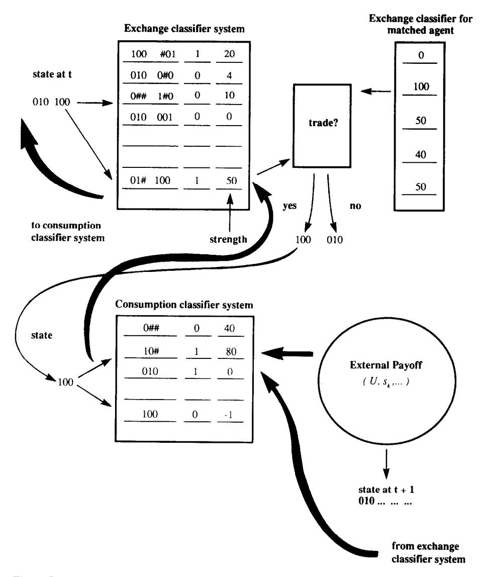
Figure 1:Example of flow of payments in classifier systems for type I agent: transfer payments denoted in bold lines, decision flows denoted in thin lines.
Figure 1 illustrates how the exchange and consumption classifier systems interact for an individual of type I. Suppose that the state at time is encoded 010 100. This means that the type I individual is storing good 2 and has been matched with someone who is storing good 1. The individual has two classifiers whose conditions are matched, one with strength 50, the other with strength 10. The strength 50 classifier makes the decision, which is ‘1’, namely, offer to trade. If the individual’s trading partner also offers to trade, the individual exits the trading process with state 100, which is the input into type I’s consumption classifier. With this input, there are two consumption classifiers whose conditions are matched, one with strength 80 that says ‘consume’, the other with strength -1 that says ‘don’t consume’. The individual consumes, initiating an external payoff. The bold lines indicate the flows of payoffs. In addition to the external payoff to the winning consumption classifier, there is a payment from the winning consumption classifier at to the winning exchange classifier at , and a payment from the winning exchange classifier at to the winning consumption classifier at .
With (14), (15), and (16), we have completed our description of the classifier system for agent when that classifier system contains a complete enumeration of possible rules. Our version of the Kiyotaki-Wright model is formed by assuming that each agent of type uses the same classifier system to make decisions.[6] Thus, we can replace superscripts and subscripts in the descriptions of strengths by ’s. We start with a set of initial strengths for . We temporarily introduce the index to index calendar time, while now temporarily indexes the cumulative number of matches which have occurred rather than calendar time. Our artificially intelligent agents then interact as follows for each , where is the length of our simulation. All agents are randomly matched into pairs. For each pair , the exchange and classifier systems for agents whose types are and , respectively, are used mutually to determine the trading and consumption decisions of agents and . After the consumption decisions have been made for the pair, the counters and the strengths of the classifier systems for both types of agents are updated according to (10), (12), (14), and (15). Also, after each pair has played, the synthetic time counter is augmented by one. After all pairs have played, the counter is augmented by one, and the entire process is repeated. The counter records the passage of physical time, while the counter records the cumulative number of matches that have occurred. The outcomes of all matches are interpreted as having occurred during period .
In 7. Simulation Results, we shall be interested in recording various frequency distributions across agents as a function of calendar time. That is, there will be distinct frequency distributions of, e.g., holdings of goods across agents for each date in calendar time. At the risk of confusion, we choose to index calendar time by (rather than ) in subsequent sections.
4. Classifier Systems for Supporting Kiyotaki and Wright’s Stationary Equilibria
4.1 The Fundamental Equilibrium
For their model A, Kiyotaki and Wright define as the fundamental equilibrium the trading pattern defined by the triangle depicted in Figure 2. In this trading pattern, good 1, which has the lowest storage cost, serves as the general medium of exchange. In terms of storage, agents of type I only store good 2, which they exchange only for good 1; agents of type III only store good 1, which they exchange only for good 3; and agents of type II half of the time store good 1, which they exchange for good 2, and half of the time good 3, which they exchange for good 1.
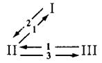
Figure 2:Exchange patterns in fundamental equilibrium of model A.
We can characterize equilibria in terms of a set of probabilities that describe holding and exchanging patterns. We define
We denote by the entire set of probabilities defined in (17) for all . Associated with Kiyotaki and Wright’s stationary equilibrium is a time-invariant . In Table 2 we display the ’s for the fundamental equilibrium of Kiyotaki and Wright’s model A.
Table 2:Equilibrium probabilities for Economy A1
(a) Probability that holds , | |||
|---|---|---|---|
0 | 1 | 0 | |
0.5 | 0 | 0.5 | |
1 | 0 | 0 |
Table 3:Joint exchange probabilities in the stationary equilibrium of Economy A1
The entry in Table 3 is the triple , representing the probability that a type agent holds , meets an agent with , and trades. Note that here denotes the joint holding-meeting-trading probability, where indexes the good held and the good of the trading partner; this differs from the conditional exchange probability defined in (17), which conditions on holding and denotes exchanging for .
Table 4:Equilibrium exchange strategies for Economy A1
Note: A question mark denotes sequential equilibrium strategies for events of zero probability. The entry in the table is the triple , representing the probability that a type agent is willing to exchange good for goods 1, 2, or 3 respectively, given that is holding .
Table 5:Consumption probabilities for Economy A1
1 | 0 | 0 | |
0 | 1 | 0 | |
0 | 0 | 1 |
Table 5 shows that in any stationary equilibrium, each type of agent consumes only its own desired good.
We now describe how the strategies that support Kiyotaki and Wright’s ‘fundamental equilibrium’ can be represented as a classifier system. For the classifiers we introduce the following additional notation. Let denote the exchange classifier for a type agent that reads ‘If I am storing good and I meet an agent with good , then my exchange decision is ’; . Similarly, specific consumption classifiers for type agents are of the form for ‘If, at the end of the exchange subperiod, I am storing good , then my consumption action is ’. For more general rules, we use the subindex to denote ‘not good ’ and to denote ‘any good’. That is, is the classifier for type I agents that reads ‘If I am storing good 2 and I meet an agent not carrying good 1, then do not trade’, and is a classifier for type I that reads ‘No matter what I am storing at the end of the exchange subperiod, do not consume’.
We can simplify the study of classifier systems by considering only a small complete set of rules. For type I agents these rules are: ; ; ; ; ; . If are the only classifiers being used by agents of type I, we can say that type I agents support the fundamental equilibrium. We can also describe classifiers for type II and type III agents that support the fundamental equilibrium. These are, for type II: ; ; ; ; ; ; and for type III: ; ; ; .
It is useful to define formally the sense in which these fixed lists of classifiers support Kiyotaki and Wright’s fundamental equilibrium. Let be a fixed set of classifiers (exchange and consumption classifiers) for agent . Let the set have no redundancies in the sense that for every state , uniquely determines actions. Then the fixed set of classifiers represents a strategy for agent defined on . We use the following definition of optimality for a fixed set of classifiers:
Definition. Given the probability distributions and fixed sets of classifiers of the other agents , for all , a fixed set of classifiers is said to be optimal for agent if there exists no other set which yields higher long-run average utility for agent .
A stationary Nash equilibrium can then be defined as follows:
Definition. A stationary Nash equilibrium is a set of probability distributions and fixed sets of classifiers , , such that:
Given and , for , is optimal for agent .
and the random matching technology imply that for all .
This definition is just an alternative representation of Kiyotaki and Wright’s definition in terms of fixed lists of classifiers.
Table 6 illustrates the sequence of events under the circumstance that the only active (i.e., auction-winning) classifiers are those that support the fundamental equilibrium for agents of type I. A natural question is whether the classifier systems of the three types of agents will actually converge to a situation in which the fundamental equilibrium of Kiyotaki and Wright is supported. Before introducing some concepts that will help us think about this question, we shall briefly describe another kind of equilibrium of Kiyotaki and Wright’s model and the kind of classifier system that could support it.
Table 6:Behavior of type I agent in a fundamental equilibrium
State | Action | Next State |
|---|---|---|
Holding good 2 | Meet agent with good 1 → Trade | Holding good 1 |
Holding good 1 | Consume → Produce good 2 | Holding good 2 |
4.2 Kiyotaki and Wright’s ‘Speculative Equilibrium’
Kiyotaki and Wright show that for their model A the trading pattern associated with a fundamental equilibrium is not the only possible one in equilibrium. They show that there can occur a speculative equilibrium with a trading pattern depicted in Figure 3.
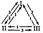
Figure 3:Exchange patterns in speculative equilibrium of Economy A.
Kiyotaki and Wright establish a condition under which the unique stationary rational-expectations equilibrium is a fundamental equilibrium. The condition, for the limiting case as the discount rate converges to zero, is that the following inequality is satisfied:[7]
In the speculative equilibrium, Table 7 depicts the flow of events in the stationary rational-expectations equilibrium for a classifier system of a type I agent. Notice that the flows depicted reduce to a set of fundamental classifiers if the dotted link is removed, i.e., if type I agents decide not to trade good 2 for good 3.
Table 7:Behavior of type I agent in a speculative equilibrium
State | Action | Next State |
|---|---|---|
Holding good 2 | Meet agent with good 1 → Trade | Holding good 1 |
Holding good 2 | Meet agent with good 3 → Trade* | Holding good 3 |
Holding good 1 | Consume → Produce good 2 | Holding good 2 |
Holding good 3 | Meet agent with good 1 → Trade | Holding good 1 |
Note: The asterisk (*) denotes the speculative move that distinguishes this from the fundamental equilibrium.
In 7. Simulation Results we shall provide an example of a simulated classifier economy where (18) is not satisfied ( is too high), but where nevertheless when agents start with a complete set of classifiers (with homogeneous strengths), the classifier systems converge to the fundamental equilibrium and not to the speculative equilibrium. Before turning to these simulations, we define some notions of stability that are designed to distinguish alternative senses in which a set of classifier systems may be said to converge.
5. Concepts of Convergence for Classifier Systems Playing Games
Given the decision rules being employed by other agents, (14)-(15) for agent forms a system of stochastic difference equations in the strengths . Since the classifier systems of the three types of agents are operating simultaneously, the behavior of the entire system is determined by the system of difference equations (14)-(15) for agent types . Let denote the strengths for an agent of type . It is natural to inquire whether the system formed by (14)-(15) for converges to a stationary point in the space of strengths, and if it does so, whether that stationary point supports the fundamental equilibrium of Kiyotaki and Wright.
Although we have not yet carried out an analysis of the convergence of this system, it seems useful at this point to report our ideas about how such an analysis could be structured. In this section we indicate how ideas from the stochastic-approximation literature might be used to study convergence in the space of strengths.[8]
From the stochastic-approximation literature,[9] we know that any limit points must satisfy
for all and . For a given we define the solutions of (20) as a stationary set of strengths for agent . Given a stationary set of strengths for agent , one can determine the set of classifiers that would win the auction for each . If has the fixed set of classifiers , where is the fixed set of classifiers that supports ’s behavior in a Nash equilibrium, then the stationary set of strengths associated with can be said to support the stationary Nash equilibrium behavior of agent .
These definitions inspire several questions. First, given stationary sets of strengths for agents of types 1, 2, 3, is it true that for a type agent, for each ? That is, does a stationary set of strengths for the classifier systems for agents of type support a stationary Nash equilibrium?
Second, given fixed sets of classifiers for of type that support a stationary Nash equilibrium, do these sets of classifiers imply the existence of a set of strengths for of type that solve (20)? That is, is every Nash equilibrium supported as a stationary point in strengths?
Third, if we let the classifier systems of agents of type run in real time, does the joint system formed by (14)-(15) for agents of each type converge almost surely, and if so, to which solution of (20) does it converge? We know from the theory of stochastic approximation that if it converges, it must converge to solutions of (20).
Associated with the third of these questions is the notion of global asymptotic stability. In future work, we plan to apply results from the stochastic approximation literature to study the global asymptotic stability of versions of our interacting classifier systems.
We also intend to study a form of stability that is distinct from and weaker than global asymptotic stability. This form of stability is summarized in the following:
Nash-like stability test. Take a stationary equilibrium fixed by . Place a single agent of a given type in the environment formed by the fixed probabilities . Let a classifier system for that single agent operate until it converges. Check to see whether it converges to imply the collection of classifiers for an agent of type which are required to support the equilibrium probabilities. In this experiment, in running the classifier system for the single agent, the decision rules of all other agents of his type are being held fixed at their equilibrium values. This experiment is to be repeated for a single agent of each type.
In the remainder of this paper, we shall not pursue the formal analysis of the stability and convergence questions formulated above.[10] Instead, we shall report computer simulations. In these computer simulations, convergence can be based either on the limiting behavior of the strengths, as indicated above, or on the convergence of key aspects of the empirical frequency distribution of holdings , which we defined in 4. Classifier Systems for Supporting Kiyotaki and Wright’s Stationary Equilibria.
6. Incomplete Enumeration Classifiers and the ‘Genetic Algorithm’
We now describe how the classifier system is modified when we deal with systems in which there is not a complete enumeration of rules. In order to complete the system, two aspects must be added to the above description of the classifier system under complete enumeration. The first is a way of generating an initial population of rules. The second is a way of deleting old rules from the system and adding new rules to the system. To generate the initial population of rules, we simply use a random number generator to generate bit strings by choosing successive bits independently.
The process of adding new rules and deleting old ones is accomplished by adding four major operations to the previous description of the workings of the classifier system. We call these steps ‘creation’, ‘diversification’, ‘specialization’, and ‘generalization’, respectively.
Creation: The creation operation is activated when there is no classifier matching the current state , i.e., is empty. In this case, a new classifier is created with its condition part defined by the current state and its action part randomly selected. A ‘weak’ classifier from the set of all classifiers is deleted to keep the number of classifiers constant.
Diversification: The diversification operation is designed to inject sufficient diversity into the range of actions called for by different classifiers in a given situation. For the exchange classifier, this step occurs at the stage at which has been observed and the set has been constructed. Recall that is the set of exchange classifiers whose condition parts match . If all have the same action (0 or 1), the diversification operation creates a classifier encoding the specific state and an action opposite to that taken by the other classifiers in . The strength of the winning classifier is assigned to this new classifier. This new classifier is added to the system, while simultaneously a ‘weak’ classifier from the set is deleted from the system. The weakness of a classifier is measured in terms of a combination of strength and cumulated number of times the classifier has won the bidding in the past. The diversification operation is used each time the classifier system is called upon. Notice that if this step were to be added to a complete enumeration system, it would have no effect on the population of rules because sufficient diversity is present from the beginning.
Specialization: The specialization operation is called randomly with a probability that we choose to be diminishing over time. The random variable governing specialization calls this step into action just after the winning bid has been determined. The winning classifier is checked to determine whether there are any 's in its condition part. A new classifier is synthesized by exposing each in the condition part to a probability of being switched to a 0 or a 1, whichever one specifically encodes the particular that was just observed or matched. This new and (probably) more specific rule is then used to replace a weak rule from the set [or in the case of the consumption classifier], where weakness is measured by a combination of strengths and cumulative number of times the auction has been won.
Generalization: The fourth step, which we call generalization, is a version of a ‘genetic algorithm’. This step is called randomly, according to a probability that we specify to be declining through time. At a point when the step is called, the process is initiated by generating two distinct populations of classifiers: ‘potential parents’ and ‘potential exterminants’. The potential parents are chosen to be a population of classifiers of specified size. They are chosen according to a ‘fitness criterion’ that weights strength and cumulative number of times that the classifier won the auction. The potential exterminants are chosen to be a population of specified size, whose members are of low fitness as measured by a fitness criterion weighting strengths and cumulative victories in past bidding.
From the population of potential parents, a specified number of pairs of parents are randomly drawn to engage in ‘mating’ for the purpose of creating children. How a pair of parents mates can be illustrated for two exchange classifiers, which are bit strings of length 7, as depicted in Figure 4.
The pair mates in two steps. First the pair draws two random integers uniformly distributed on . The two integers signify the positions between bits depicted in Figure 4. Next, a Bernoulli random variable with probability 0.5 is drawn, assuming values of ‘in’ or ‘out’. If ‘in’ is drawn, we focus on the bits between the two lines, i.e., the bits inside the randomly drawn interval. If ‘out’ is drawn, we focus on the bits outside the randomly drawn interval. Within the interval of focus, we complete the mating process via the following version of genetic crossover. For each of the parent strings in the area of focus, we change to a any bits for which the parent strings disagree. (Here, agrees with either 0 or 1, while 0 disagrees with 1). This process produces two children. The children are each assigned strengths that are the average of their parents’ strengths. The children are introduced into the population of classifiers. For each child added to the population, a randomly selected individual from the population of ‘potential exterminants’ is deleted from the population.
This completes our description of the algorithm to be used for updating the classifier system when we deal with an incomplete enumeration classifier system. In the simulations to be reported in 7. Simulation Results, we shall employ both complete and incomplete enumeration classifier systems.
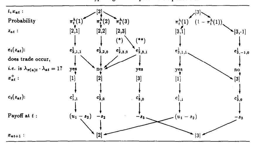
Figure 4:The mating process for exchange classifiers who have drawn ‘3,6’ and ‘in’.
7. Simulation Results
The sets of parameters defining the economies under study are summarized in Table 8.
Table 8:Description of the economies
Economy | Production | Storage costs | Utility | Initial CS | Equil. type |
|---|---|---|---|---|---|
A1.1 | 2 | F | F | ||
A1.2 | 2 | R | F | ||
A2.1 | 2 | F | S | ||
A2.2 | 2 | R | S | ||
B.1 | 3 | F | F/S | ||
B.2 | 3 | R | F/S | ||
C | 2 | R | F | ||
D | 3 | R | — |
Notes: Utility levels are set equal for . CS denotes ‘classifier system’. ‘F’ implies fixed enumeration and ‘R’ implies randomly generated rules.
7.1 Economy A1
Table 9:Parameter values used for Economy A1.1
Parameter | Value |
|---|---|
No. of agents | |
No. of classifiers | |
Storage costs | |
Utility | |
Initial strengths | |
Bids |
Economy A1.1 (Economy A1 with complete enumeration of classifiers) shows that the distribution of holdings rapidly converges to the stationary equilibrium distributions. Similarly, the exchange and consumption strategies implemented by the system of winning classifiers virtually coincide with the equilibrium strategies. In Table 10, and in all subsequent tables of empirical frequencies, the frequencies reported are ten-period moving averages ending at the indicated time periods.[11]
Table 10:Frequency with which holds at and for Economy A1.1
() | 0 | 1 | 0 |
() | 0.502 | 0 | 0.498 |
() | 1 | 0 | 0 |
() | 0 | 1 | 0 |
() | 0.506 | 0 | 0.494 |
() | 1 | 0 | 0 |
Table 11:Exchange frequency at and for Economy A1.1
() | |||
() | |||
() | |||
() | |||
() | |||
() |
Table 12:Winning classifier actions at for Economy A1.1
— | — | ||
— | |||
— | — |
Table 13:Highest-strength consumption classifiers for type I at , Economy A1.1
Iteration | Classifier | Strength |
|---|---|---|
1000 | 1 0 0 1 | 45.8 |
# # 0 0 | −0.47 | |
0 # # 1 | −9.16 |
Table 14:Highest-strength exchange classifiers for type I at , Economy A1.1
Iteration | Classifier | Strength |
|---|---|---|
1000 | 0 # # 1 0 0 1 | 11.22 |
0 # # 0 1 0 0 | −0.08 | |
# # 0 0 0 1 0 | −0.08 |
Table 15:Highest-strength consumption classifiers for type II at , Economy A1.1
Iteration | Classifier | Strength |
|---|---|---|
1000 | 1 0 0 0 | 0.0089 |
0 1 0 1 | 49.04 | |
# 0 # 0 | −10.90 |
Table 16:Highest-strength exchange classifiers for type II at , Economy A1.1
Iteration | Classifier | Strength |
|---|---|---|
1000 | # # 0 # # 0 1 | 4.86 |
# # 0 # 0 # 0 | 0.002 | |
0 0 1 1 0 0 1 | 0.002 | |
0 # # 0 1 0 1 | 12.72 | |
0 # # 0 # # 0 | −1.79 |
Table 17:Highest-strength consumption classifiers for type III at , Economy A1.1
Iteration | Classifier | Strength |
|---|---|---|
1000 | # 0 # 0 | −0.024 |
# # 0 0 | −0.412 | |
0 0 1 1 | 31.62 |
Table 18:Highest-strength exchange classifiers for type III at , Economy A1.1
Iteration | Classifier | Strength |
|---|---|---|
1000 | # 0 # # 0 # 1 | −0.01 |
# 0 # 0 1 0 0 | −0.01 | |
# 0 # 0 0 1 1 | 7.78 |
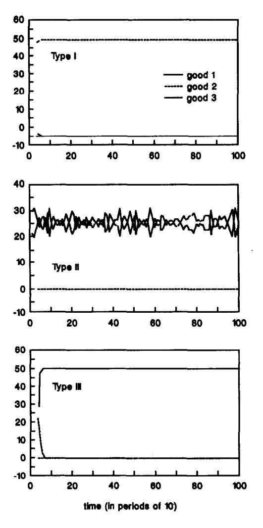
Figure 5:Distribution of holdings for Economy A1.1.
Table 19:Parameter values used for Economy A1.2
Parameter | Value |
|---|---|
No. of agents | |
No. of classifiers | |
Storage costs | |
Utility | |
Initial strengths | |
Bids | |
Specialization | |
Generalization |
Economy A1.2 is identical to Economy A1.1, except that we use a randomly generated list of rules initially, and rely on a genetic algorithm to inject new rules into the classifier’s system.[12]
Table 20:Frequency with which holds at and for Economy A1.2
() | 0 | 0.992 | 0.008 |
() | 0.226 | 0 | 0.774 |
() | 1 | 0 | 0 |
() | 0 | 0.98 | 0.02 |
() | 0.318 | 0 | 0.682 |
() | 1 | 0 | 0 |
Table 21:Exchange frequency at and for Economy A1.2
() | |||
() | |||
() | |||
() | |||
() | |||
() |
Table 22:Winning classifier actions at and for Economy A1.2
() | |||
|---|---|---|---|
() | |||
— |
Table 23:Consumption frequency at and for Economy A1.2
() | 1 | 0.011 | 0.049 |
() | 0.45 | 1 | 0.366 |
() | 0.033 | — | 1 |
() | 1 | 0 | 0.69 |
() | 0.23 | 1 | 0.641 |
() | 0.84 | 1 | 1 |
Table 24:Highest-strength consumption classifiers for type I, Economy A1.2
Iteration | Classifier | Strength |
|---|---|---|
1000 | 1 0 0 1 | 38.11 |
0 1 # 0 | −0.44 | |
0 0 1 1 | −4.26 | |
2000 | 1 0 0 1 | 41.65 |
0 1 0 0 | −0.43 | |
0 0 1 0 | −8.86 |
Table 25:Highest-strength exchange classifiers for type I, Economy A1.2
Iteration | Classifier | Strength |
|---|---|---|
1000 | 0 1 0 1 0 0 1 | 8.27 |
0 1 0 0 1 0 1 | −0.09 | |
0 1 0 0 0 1 0 | −0.10 | |
2000 | 0 1 0 1 0 0 1 | 9.05 |
0 1 0 0 1 0 0 | −0.10 | |
0 1 0 0 0 1 1 | −0.10 |
Table 26:Highest-strength consumption classifiers for type II, Economy A1.2
Iteration | Classifier | Strength |
|---|---|---|
1000 | # # 0 0 | 1.88 |
0 # 0 1 | 11.48 | |
0 0 1 1 | −9.29 | |
2000 | # # 0 0 | 8.05 |
0 # 0 1 | 38.40 | |
0 0 1 1 | −9.01 |
Table 27:Highest-strength exchange classifiers for type II, Economy A1.2
Iteration | Classifier | Strength |
|---|---|---|
1000 | 1 0 0 1 0 0 0 | 0.29 |
1 0 0 0 1 0 1 | 1.67 | |
1 0 0 0 0 1 0 | 0.28 | |
0 0 1 # # 0 1 | 2.23 | |
0 # 1 0 1 0 0 | 4.08 | |
0 0 1 0 0 1 1 | −2.08 | |
2000 | 1 0 0 1 0 0 0 | 1.32 |
1 0 0 0 1 0 1 | 6.15 | |
1 0 0 0 0 1 0 | 1.25 | |
0 0 1 1 0 0 1 | 1.34 | |
0 # 1 0 1 0 1 | 2.98 | |
0 0 1 0 0 1 1 | −1.99 |
Table 28:Highest-strength consumption classifiers for type III, Economy A1.2
Iteration | Classifier | Strength |
|---|---|---|
1000 | 1 0 0 0 | 0.00 |
0 0 1 1 | 30.94 | |
2000 | 1 0 0 1 | 8.97 |
0 0 1 1 | 30.55 |
Table 29:Highest-strength exchange classifiers for type III, Economy A1.2
Iteration | Classifier | Strength |
|---|---|---|
1000 | 1 0 0 # # # 0 | 0.28 |
1 0 0 0 # # 0 | 1.77 | |
1 # # 0 # 1 1 | 7.39 | |
2000 | 1 0 0 1 # 0 0 | 0.14 |
1 0 0 0 1 0 1 | 0.42 | |
1 # # 0 # 1 1 | 7.25 |
As we can see from Figure 6 and the above tables, the distribution of holdings for agents of type I and III rapidly converge to their equilibrium levels. Type II agents only hold goods 1 and 3 as predicted but it takes longer to converge to the equilibrium values. The exchange decisions are the correct ones (even in period 1000), except for a couple of events of very small probability (type I agents trade good 2 for 3 and type III agents trade good 1 for 2).
Consumption decisions are basically correct, except that II consumes 3 and III consumes 1. Overeating has been a minor problem in several of our economies. In most such cases that we have encountered, such wrong behavior has been associated with low-frequency states for which it is difficult for the classifier system to acquire the experience required to reward better classifiers and ‘right’ actions.
In summary, both with complete enumeration and without it, our simulations of Economy A1 seem to be converging to the stationary equilibrium, although this convergence is slower when initial classifiers are randomly generated and new classifiers are synthesized.
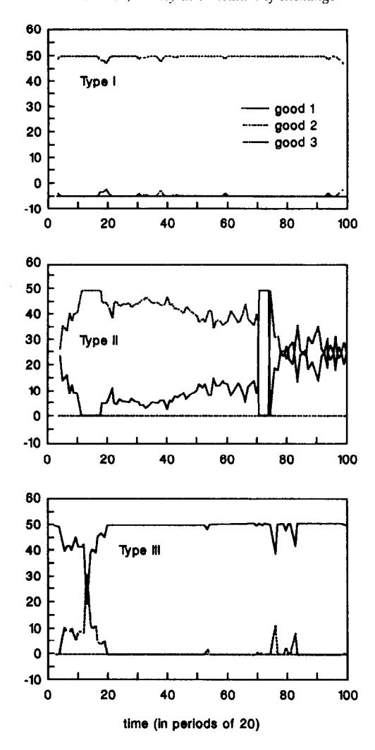
Figure 6:Distribution of holdings for Economy A1.2.
7.2 Economy A2
Table 30:Parameter values used for Economy A2.1
Parameter | Value |
|---|---|
No. of agents | |
No. of classifiers | |
Storage costs | |
Utility | |
Initial strengths | |
Bids |
Economy A2 differs from Economy A1 only in that agents receive 500 utils from consuming their desired good instead of 100. With this change of parameters, for high enough discount factors the unique stationary equilibrium of Kiyotaki and Wright’s economy is the so-called speculative equilibrium. The probabilities that characterize the speculative equilibrium are summarized in Table 31.
Table 31:Speculative equilibrium: probability that holds , , for Economy A2
0 | 0.707 | 0.293 | |
0.586 | 0 | 0.414 | |
1 | 0 | 0 |
Table 32:Speculative equilibrium: joint exchange probability for Economy A2
Table 33:Speculative equilibrium exchange strategies for Economy A2
Table 34:Frequency with which holds at and for Economy A2.1
() | 0 | 1 | 0 |
() | 0.504 | 0 | 0.496 |
() | 1 | 0 | 0 |
() | 0 | 1 | 0 |
() | 0.466 | 0 | 0.534 |
() | 1 | 0 | 0 |
Table 35:Exchange frequency at and for Economy A2.1
() | |||
() | |||
() | |||
() | |||
() | |||
() |
Table 36:Winning classifier actions at and for Economy A2.1
() | |||
|---|---|---|---|
() | |||
Table 34 depicts a pattern of holdings characteristic of a fundamental equilibrium, not a speculative one. Compare with the theoretical predictions of Table 31–Table 32. Recall that a crucial difference between a speculative and a fundamental equilibrium is that in the former, type I agents are willing to exchange good 2 for good 3, while in the latter they are not. Table 36 shows that type I agents are willing to exchange good 2 for 3, i.e., for . Then how is it that the distribution of holding patterns fails to support a speculative equilibrium? The answer is to be found in the consumption classifiers of type I agents, which are too general (have too many signs) to distinguish among goods stored. It happens that the winning classifiers embody levels of generality that result in overconsumption of good 3 and a failure to transmit the information from the consumption classifier to the exchange classifier that would be required to support a speculative equilibrium.[13]
We shall only briefly summarize the results for Economy A2.2 with random generation of initial classifiers, and refer the reader to the working paper for tables giving the numerical results. After 1000 iterations the economy had not converged to a steady state. Trading patterns were closer to the fundamental equilibrium than to the speculative equilibrium in period 1000. (The reverse was true in period 500.) However, the classifier system of type I agents did distinguish between storage of different goods for consumption, and the classifier was slowly gaining strength over time. Nevertheless, our simulations provided no support for a hope that the economy would converge to the speculative equilibrium if it were to last longer.
While the results for Economy A2 are fairly inconclusive, they illustrate two interesting points. First, they expose some deficiencies of the genetic algorithm which we have used (we return to this in 8. Conclusions). Second, they raise the issue of whether our artificially intelligent agents are too impatient.
Patience requires experience. The transfer system inside the classifier system is designed to converge to a set of long-run average strengths. In the limit, the artificially intelligent agents should behave as long-run average payoff maximizers, since the steady-state strengths weight payoffs by their relative frequencies. It takes time, however, for optimal rules to achieve the desired strengths. The behavior of our artificially intelligent agents can be very myopic at the beginning. In economies, such as Economy A2, in which the nature of the equilibrium changes with the discount rate, this early myopia might have a perverse effect in diverting the economy towards a low discount-factor stationary equilibrium, such as the fundamental equilibrium. The underlying algorithm has to provide enough experimentation to avoid an early ‘lock in’.[14][15] The present algorithm seems defective in that it has too little experimentation to support the speculative equilibrium even in the long simulations we have run.
7.3 Economy B
Table 37:Parameter values used for Economy B.1
Parameter | Value |
|---|---|
No. of agents | |
No. of classifiers | |
Storage costs | |
Utility | |
Initial strengths | |
Bids |
Economy B has a different production pattern than Economy A (I produces 3, II produces 1, and III produces 2). For the specified parameters two stationary equilibria are possible: fundamental and speculative. Stability tests based on classifier systems are potentially useful as selection criteria in economies with multiple equilibria. Table 38 and Table 41 summarize the trading patterns for the fundamental and the speculative equilibrium, respectively.
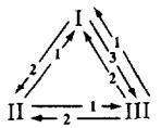
Figure 7:Exchange patterns in Economy B: Fundamental Equilibrium (left) and Speculative Equilibrium (right).
Table 38:Fundamental equilibrium: probability that holds , , for Economy B
0 | 0.293 | 0.707 | |
1 | 0 | 0 | |
0.586 | 0.414 | 0 |
Table 39:Fundamental equilibrium: joint exchange probability for Economy B
Table 40:Fundamental equilibrium exchange strategies for Economy B
Table 41:Speculative equilibrium: probability that holds , , for Economy B
0 | 0.586 | 0.414 | |
0.707 | 0 | 0.293 | |
0 | 1 | 0 |
Table 42:Speculative equilibrium: joint exchange probability for Economy B
Table 43:Speculative equilibrium exchange strategies for Economy B
Economy B.1 displays an interesting pattern of evolution. At iteration 500 the distribution of holdings and, especially, the trading patterns correspond to the speculative equilibrium. However, the economy moves away from this state and by iteration 1000 has practically converged to the fundamental equilibrium.
Table 44:Frequency with which holds at and for Economy B.1
() | 0 | 0.464 | 0.536 |
() | 0.994 | 0 | 0.006 |
() | 0 | 1 | 0 |
() | 0 | 0.28 | 0.72 |
() | 0.994 | 0 | 0.006 |
() | 0.526 | 0.474 | 0 |
Table 45:Exchange frequency at and for Economy B.1
() | |||
() | |||
() | |||
() | |||
() | |||
() |
Table 46:Winning classifier actions at and for Economy B.1
() | |||
|---|---|---|---|
() | |||
Table 47:Consumption frequency at for Economy B.1
1 | 0.07 | 0.508 | |
0.009 | 1 | 0.998 | |
0.050 | 0.632 | 1 |
Economy B.2 with random initial classifiers had not converged after 2000 periods. Nevertheless, the economy seems to be moving towards the fundamental equilibrium.
Table 48:Parameter values used for Economy B.2
Parameter | Value |
|---|---|
No. of agents | |
No. of classifiers | |
Storage costs | |
Utility | |
Initial strengths | |
Bids | |
Specialization | |
Generalization |
Table 49:Frequency with which holds at and for Economy B.2
() | 0 | 0.434 | 0.566 |
() | 0.89 | 0 | 0.11 |
() | 0.088 | 0.912 | 0 |
() | 0 | 0.354 | 0.646 |
() | 0.996 | 0 | 0.004 |
() | 0.268 | 0.732 | 0 |
Table 50:Exchange frequency at and for Economy B.2
() | |||
() | |||
() | |||
() | |||
() | |||
() |
Table 51:Winning classifier actions at and for Economy B.2
() | |||
|---|---|---|---|
— | |||
() | |||
— |
In particular, with the exception of a zero-frequency event (II is willing to trade 1 for 3) the trading patterns in Economy B.2 correspond to the fundamental equilibrium.
These two simulations for Economy B provide examples in which the classifier systems seem to select the fundamental equilibrium over the speculative equilibrium.[16] Furthermore, the results for Economy B.1 indicate that this is not the result of myopic behavior.
7.4 Economy C (Fiat Money)
Table 52:Parameter values used for Economy C
Parameter | Value |
|---|---|
No. of agents | |
No. of classifiers | |
Storage costs | |
Utility | |
Initial strengths | |
Bids | |
Specialization | |
Generalization |
In Economy C a new good, good 0, with the characteristics of ‘fiat money’ is introduced. No agent derives utility from consuming good 0. There are no storage costs associated with good 0.
Fiat money is introduced into the system by forcing some agents to store good 0 in period 0. In particular, 48 units of good 0 are randomly allocated to 48 agents. To avoid fluctuations in the quantity of money, agents are not allowed to consume good 0. A modified setup, not pursued here, would give agents the opportunity to learn not to eat money.
The production technologies are as in Economy A (see Table 8). Table 53 provides the probabilities that characterize the unique (fundamental) equilibrium of Economy C. The equilibrium trading patterns are depicted in Figure 8.
Table 53:Fundamental equilibrium: probability that holds , , for Economy C
0 | 0.26 | 0.62 | |
0.74 | 0 | 0 | |
0 | 0.42 | 0 | |
0.26 | 0.32 | 0.38 |
Table 54:Fundamental equilibrium: joint exchange probability for Economy C
Table 55:Fundamental equilibrium exchange strategies for Economy C
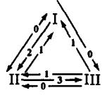
Figure 8:Exchange pattern in Economy C.
Table 56:Frequency with which holds at and for Economy C
() | 0 | 0.18 | 0.58 |
() | 0.68 | 0 | 0.01 |
() | 0 | 0.58 | 0 |
() | 0.32 | 0.23 | 0.41 |
() | 0 | 0.18 | 0.77 |
() | 0.54 | 0 | 0.01 |
() | 0 | 0.53 | 0 |
() | 0.46 | 0.28 | 0.21 |
Table 57:Exchange frequency at for Economy C
Table 58:Exchange frequency at for Economy C
Table 59:Winning classifier actions at and for Economy C
() | |||
|---|---|---|---|
() | |||
The economy converges remarkably fast to the fundamental equilibrium. Given the complexity of the exchange patterns with fiat money, the results for Economy C indicate the ability of our artificially intelligent agents to set up complex social arrangements like fiat money.[17]
7.5 Economy D (Five Goods, Five Types)
Table 60:Parameter values used for Economy D
Parameter | Value |
|---|---|
No. of agents | |
No. of classifiers | |
Storage costs | |
Utility | |
Initial strengths | |
Bids | |
Specialization | |
Generalization |
In Economy D we enhance complexity by considering five goods and five types. The production technologies are described by Figure 9. That is, type I produces good 3, type II produces good 4, type III produces good 5, type IV produces good 1, and type V produces good 2. As before, each type of agent only derives utility from consuming the good of the same number. Storage costs are ranked in increasing order. For this economy we do not start with any characterization of a stationary equilibrium. With enough work, one could obtain an analytic solution for the fundamental equilibrium for such an economy, but here our purpose is to let our artificially intelligent agents suggest to us what an equilibrium might be. Given this suggestion, we could then presumably verify whether it is an equilibrium.
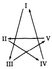
Figure 9:Production patterns in Economy D; an arrow shows that the agent at the origin of the arrow produces the good at the point of the arrow.
Table 61:Frequency with which holds at for Economy D
0 | 0.336 | 0.626 | 0.032 | 0.006 | |
0.322 | 0 | 0.038 | 0.614 | 0.026 | |
0.118 | 0.180 | 0 | 0.054 | 0.648 | |
0.922 | 0.044 | 0.002 | 0 | 0.032 | |
0.210 | 0.720 | 0.038 | 0.032 | 0 |
Table 62:Frequency with which holds at for Economy D
0 | 0.832 | 0.158 | 0.004 | 0.006 | |
0.096 | 0 | 0.004 | 0.870 | 0.030 | |
0.048 | 0.418 | 0 | 0.052 | 0.482 | |
0.988 | 0.008 | 0.002 | 0 | 0.002 | |
0 | 0.974 | 0.024 | 0.002 | 0 |
Table 63:Exchange frequency at for Economy D
Table 64:Exchange frequency at for Economy D
Table 65:Winning classifier actions at for Economy D
Table 66:Winning classifier actions at for Economy D
From the simulation results, we can see that the trading patterns nearly seem to describe a fundamental equilibrium in which agents are only willing to trade for commodities of lower cost than the one currently in storage, except that they always accept the commodity of their type. These fundamental trading patterns are shown in Figure 10. Some speculative moves can be detected. An example of this is that agents of type II accept (from I) good 3 for good 1 in order to trade 3 for 2 with type III. We do not pursue here a full analysis of partially speculative equilibria for this economy.
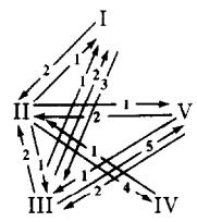
Figure 10:Exchange patterns in Economy D exhibited by classifier systems.
8. Conclusions
The work described above is presented as the first steps of our project to use the classifier systems of Holland to model learning in multi-agent environments. Classifier systems have previously been applied to solve some complex optimization problems [see Machine Learning (1988)]. Our application has involved some extensions to handle the fact that ours is a multi-agent environment in which agents are solving Markovian dynamic decision problems.
The work described in this paper has accomplished two objectives that are parts of our broader project. First, our simulations have demonstrated by example that multi-agent systems of classifiers can exhibit interesting behavior, and can eventually learn to play Nash-Markov equilibria. Second, the process of making classifier systems cope with the Kiyotaki-Wright environment has prompted us to formalize a variety of concepts and definitions that our subsequent work shall build on. These definitions will facilitate formal analyses of systems of multi-agent classifier systems, which we intend to pursue.
Among the unfinished aspects which we leave for future papers, two interrelated ones are quite important. First, our experiments with the genetic-type algorithms in our incomplete-enumeration classifier systems have convinced us that existing algorithms can be improved. These improvements, which will increase the amount of experimentation that is done at the ‘right times’, will have the effect of improving the capacity of the classifier systems to settle upon optimal outcomes more rapidly, and to avoid becoming locked in to suboptimal patterns of interaction. The improved algorithms will also help with a second major piece of unfinished business, which is to develop analytical results on the convergence of classifier systems. The new algorithms will be set up in such a way that we can apply the stochastic approximation approach to convergence analysis which we alluded to in 5. Concepts of Convergence for Classifier Systems Playing Games.
References
Acknowledgments
This research began with visits by Marimon and Sargent to the Santa Fe Institute. We thank Brian Arthur and John Holland for several helpful discussions about genetic algorithms at the Santa Fe Institute. We also thank Randall Wright and Nancy Stokey for helpful comments on an earlier draft. Sargent’s research was supported by a grant from the National Science Foundation to the National Bureau of Economic Research. Marimon’s research was supported by a grant from the National Science Foundation and by the National Fellows Program at the Hoover Institution. This paper is an abbreviated version of a Hoover Institution working paper with the same title, which is available from the authors upon request.
The way in which we model agents as searching for rewarding decision rules attributes much less knowledge and rationality to them than is typical in the literature on least-squares learning in the context of linear rational-expectations models. See Bray (1982), Bray & Savin (1986), Fourgeaud et al. (1986), and Marcet & Sargent (1989). In the least-squares learning literature, agents are posited to be almost fully rational and knowledgeable about the system they operate within, lacking knowledge only about particular parameters in laws of motion of a set of variables exogenous to their own decisions, which they learn about through the recursive application of least squares. But given their estimates, agents are supposed to compute optimal decision rules by using dynamic programming or the calculus of variations.
When the state and action spaces are small, as in the Kiyotaki-Wright model, the list of all possible rules mapping states into actions is not too long. In such a situation, one can follow Axelrod (1987) and model an agent’s strategy as a single binary bit string. A pure genetic algorithm can then be applied, as in Axelrod (1987). This approach has been applied to the Kiyotaki-Wright model by Marimon and Miller (1989) and by Knez and Litterman (1989). While much easier to implement than classifier systems, this pure genetic approach also has some drawbacks. First, it is difficult to extend to situations involving ‘unforeseen contingencies’ and in which it is not practical to enumerate all of the histories that might be encountered in the course of play. Second, relative to the classifier, the pure genetic algorithm encodes information wastefully in the sense that an entire strategy is encoded, while the experience of play will typically throw up observations only on a small subset of the possible states. While the classifier system concentrates ‘effort’ on learning rules to use in frequently encountered states, the pure genetic algorithm purports to be learning about entire strategies. Third, classifiers can learn general rules that apply to several states and that offer potential informational economies.
A pure genetic algorithm could be applied to the trading decision as follows. For each agent, there are possible values that his current state prior to trade can attain. There are two possible actions: trade or don’t trade. Letting 1 mean trade and 0 mean don’t trade, a binary string of length 9 can be used to encode a Markovian strategy. This is done by numbering the set of possible states and then letting the th entry in the bit string denote the decision to be made when the th state is encountered. The genetic algorithm is then applied to select the best binary string (i.e., the best strategy). This approach, which has been applied to the Kiyotaki-Wright model [see Marimon and Miller (1989) and Knez and Litterman (1989)], has shortcomings as a starting point for studying more complex systems. Because the optimization is done over entire strategies, which include descriptions of decisions to be made in all possible states, even rarely visited ones, the encoding of information is wasteful and does not facilitate more intensive learning about frequently visited states.
See Goldberg (1989) for a description of classifier systems and a survey of some of their applications.
This rule could easily be modified to permit a ‘stochastic auction’ in which the probability of winning the auction varies directly with strength.
We make this specification in order to economize on computer time and space. It is possible that this specification speeds convergence relative to a setting in which each agent uses his own classifier system. However, relative to a setup in which each agent uses his own classifier system and so can experiment individually, the common classifier setup causes all type agents to experiment simultaneously. This feature might delay convergence.
Notice that this condition involves both parameter values (, , ) and the quantities (, ) which are endogenous variables that are determined in equilibrium. Kiyotaki and Wright show that when the above inequality is reversed, then the unique stationary rational-expectations equilibrium is a speculative equilibrium. Vis-à-vis the fundamental equilibrium, the only change in trading patterns is that agents of type I ‘speculate’ by holding good 3, which is not too costly because in equilibrium inequality (18) is reversed.
It was considerations from the stochastic-approximation literature that led us to alter Holland’s specification of the laws of motion of strengths so that they measure cumulative average past net rewards, not total rewards. The use of average rewards makes it possible for strengths to converge. Arthur (1989) uses average rewards for strengths for the same reason.
Ljung & Söderström (1983) is a useful reference on stochastic approximation and on the ‘ordinary differential-equations approach’ to proving almost sure convergence. See Marcet & Sargent (1989) and Marcet & Sargent (1989) for some applications in economics.
Brian Arthur and Carl Simon have used stochastic approximation arguments to establish convergence of strengths for a fixed system of two classifiers playing a two-armed bandit. Their arguments do not apply to our system because their system is one in which there are competing classifiers with distinct actions, whose condition parts are identical and are always met.
When ‘—’ appears in the table, it means that the event in question occurred so rarely in our simulation that no reliable frequency can be computed.
More standard Holland algorithms were first tried without much success, prompting us to produce the modified algorithm described in 6. Incomplete Enumeration Classifiers and the ‘Genetic Algorithm’.
To conserve space, these classifiers are not reported here. They are contained in a longer version of this paper which is available from the authors as a working paper.
A fundamental equilibrium exists for Economy A2 only if the discount factor is sufficiently low.
Marimon and Miller (1989) report that in their experiments with the genetic algorithm 25 out of 30 runs of Economy A2 converged to the speculative equilibrium.
In Marimon and Miller (1989) 30 out of 30 experiments resulted in convergence to the fundamental equilibrium.
A version of Economy C with the storage costs of Economy A did not converge, probably because the low cost of storing good 1 (0.1) made this good too good a substitute for fiat money. These results for Economy C have been successfully replicated in Marimon and Miller (1989).
- Kiyotaki, N., & Wright, R. (1989). On Money as a Medium of Exchange. Journal of Political Economy, 97(4), 927–954.
- Holland, J. H. (1975). Adaptation in Natural and Artificial Systems. University of Michigan Press.
- Holland, J. H. (1986). Escaping Brittleness: The Possibilities of General-Purpose Learning Algorithms Applied to Parallel Rule-Based Systems. In R. S. Michalski, J. G. Carbonell, & T. M. Mitchell (Eds.), Machine Learning: An Artificial Intelligence Approach (Vol. 2). Morgan Kaufmann.
- Machine Learning. (1988). Special Issue on Genetic Algorithms. Machine Learning, 3(2/3).
- Bray, M. (1982). Learning, Estimation, and Stability of Rational Expectations. Journal of Economic Theory, 26, 318–339.
- Bray, M. M., & Savin, N. E. (1986). Rational Expectations Equilibria, Learning and Model Specification. Econometrica, 54, 1129–1160.
- Fourgeaud, C., Gourieroux, C., & Pradel, J. (1986). Learning Procedure and Convergence to Rationality. Econometrica, 54, 845–868.
- Marcet, A., & Sargent, T. J. (1989). Convergence of Least Squares Learning Mechanisms in Self Referential Linear Stochastic Models. Journal of Economic Theory, 48, 337–368.
- Axelrod, R. (1987). The Evolution of Strategies in the Iterated Prisoner’s Dilemma. In L. Davis (Ed.), Genetic Algorithms and Simulated Annealing. Morgan Kaufmann.
- Goldberg, D. E. (1989). Genetic Algorithms in Search, Optimization and Machine Learning. Addison-Wesley.
- Arthur, B. (1989). The Dynamics of Classifier Competitions.
- Ljung, L., & Söderström, T. (1983). Theory and Practice of Recursive Identification. MIT Press.
- Marcet, A., & Sargent, T. J. (1989). Convergence of Least Squares Learning in Environments with Private Information and Hidden State Variables. Journal of Political Economy, 97, 1306–1322.